Simulating Conductive Electrodes with the Constant Potential Method
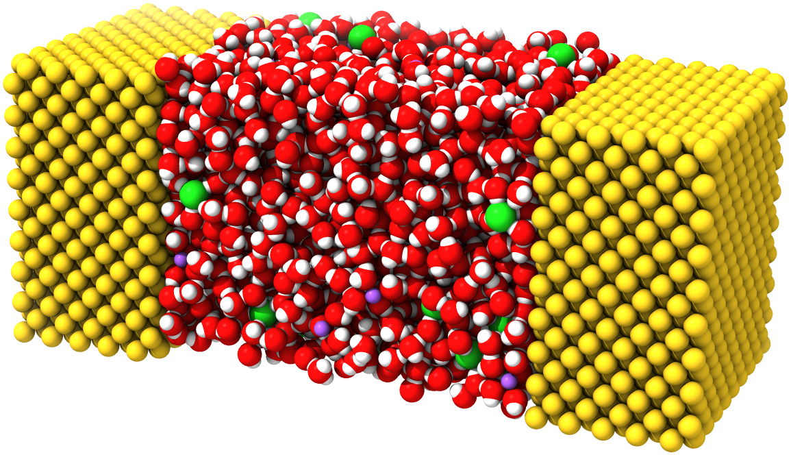
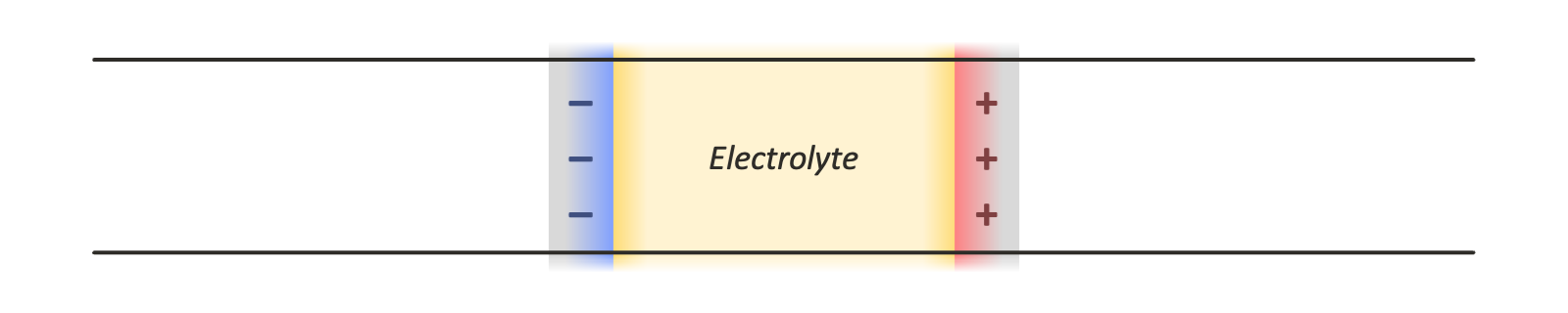
The constant potential molecular dynamics method is an approach for simulating conductive materials with delocalized charges, and maintaining them at prescribed electric potentials. In constant potential simulations, the charges on a prescribed set of particles (those belonging to the conductive material, or the “electrode particles”) are allowed to fluctuate as they interact with other particles in the system. This is useful for studying various kinds of electrochemical systems, e.g., the electrode-electrolyte interface in a parallel plate capacitor. In this tutorial, we will show how to set up a constant potential simulation using OpenMM’s implementation of this method. Specifically, we will use a capacitor system described in Ref. 1, with an aqueous NaCl electrolyte sandwiched between two Au electrodes:
Theory
A full exposition of the theory behind constant potential simulations is beyond the scope of this tutorial, but it is useful to be acquainted with the basics before getting started. In ordinary molecular simulations with fixed charges, we wish to sample configurations \(\mathbf{r}^N\) of \(N\) particles based on some potential energy function \(U(\mathbf{r}^N)\). In the constant potential approach, some number \(M\) of particles are allowed to have varying charges, so that we have \(U(\mathbf{r}^N,\mathbf{q}^M)\). The commonly used method implemented by OpenMM for constant potential simulations uses a Born-Oppenheimer-like approach in which \(\mathbf{q}^M\) is chosen at every step to minimize \(U\) for the given \(\mathbf{r}^N\). Since electrostatic interactions can be treated with Coulomb’s law, \(U\) is quadratic in the \(\mathbf{q}^M\), and minimizing it is equivalent to solving a linear system.
Actually computing the coefficients of this system, which are functions of the particle positions, is more complex. For parallel plate capacitor geometries like the one shown above, the system effectively has periodic boundary conditions in the plane of the electrodes, but is non-periodic in the direction normal to their surfaces.
There are a few options for using periodic boundary conditions in all three dimensions so that standard tools for computing the electrostatic interactions, such as the particle mesh Ewald method, can be employed. Leaving empty space between periodic images introduces various complications, since this effectively creates a pair of dissimilar capacitors, one containing an electrolyte material of interest, and another containing vacuum. Another option is a double cell geometry, with each periodic image containing the capacitor system of interest and a reflected copy of it. This keeps the net potential difference across the simulation cell, and its net dipole moment, zero:
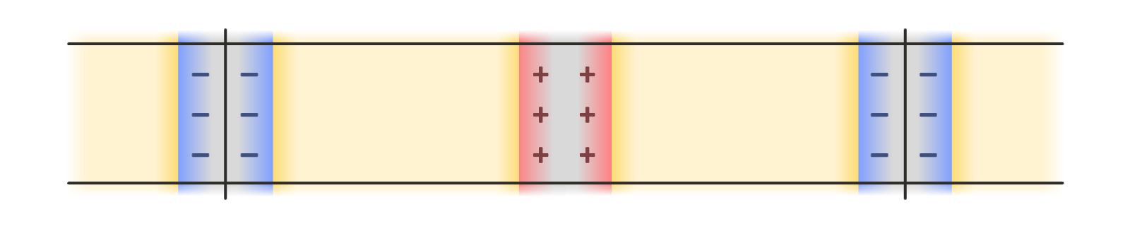
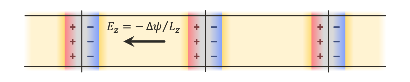
The implementation in OpenMM supports such geometries, but they are more computationally expensive, requiring double the number of particles in the system of interest. In this tutorial, we show how to use the finite field method described in Ref. 2, in which only a single copy of the system is needed, and an external electric field is applied to all charges in the system to maintain the desired electric potential difference across the periodic box:
There are many more details that this tutorial will not explore, but the reader is referred to Refs. 1-3 for more information about the theory, as well as to the user guide for the details of the specific implementation in OpenMM.
Setting Parameters
To begin writing a script implementing our capacitor system in OpenMM, we will import OpenMM (as well as NumPy, which is just used to read in the initial coordinates for this example).
[1]:
import openmm
import openmm.app
import openmm.unit

import numpy as np
We now define various parameters for the simulation. An appropriate geometry, force field, and parameters for a constant potential simulation will depend on the system you are interested in; here, we use data provided with the work of Ref. 1. We begin with the periodic box dimensions for the simulation:
[2]:
L_XY = 69.2206679755 * openmm.unit.bohr
L_Z = 204.0 * openmm.unit.bohr
VECTORS = (
    (L_XY, 0.0 * openmm.unit.bohr, 0.0 * openmm.unit.bohr),
    (0.0 * openmm.unit.bohr, L_XY, 0.0 * openmm.unit.bohr),
    (0.0 * openmm.unit.bohr, 0.0 * openmm.unit.bohr, L_Z),
)
The electrolyte between the plates contains 2160 water molecules and 39 NaCl ion pairs. Each electrode contains 1620 gold atoms:
[3]:
N_WATER = 2160
N_NACL = 39
N_AU = 1620
We now define some standard parameters for each of the atom types:
[4]:
# Atom masses:
M_H = 1.008 * openmm.unit.dalton
M_O = 15.9994 * openmm.unit.dalton
M_NA = 22.9898 * openmm.unit.dalton
M_CL = 35.453 * openmm.unit.dalton

# Lennard-Jones energy scales:
EPS_O = 0.6502 * openmm.unit.kilojoule_per_mole
EPS_NA = 0.4184 * openmm.unit.kilojoule_per_mole
EPS_CL = 0.4184 * openmm.unit.kilojoule_per_mole
EPS_AU = 22.13336 * openmm.unit.kilojoule_per_mole

# Lennard-Jones length scales:
SIG_O = 3.166 * openmm.unit.angstrom
SIG_NA = 2.584 * openmm.unit.angstrom
SIG_CL = 4.401 * openmm.unit.angstrom
SIG_AU = 2.951 * openmm.unit.angstrom

# H atom charge for water:
Q_H = 0.4238 * openmm.unit.elementary_charge
This simulation uses the rigid 3-site SPC/E water model; the distances between its atoms are as follows:
[5]:
L_OH = 1.88972 * openmm.unit.bohr
L_HH = 3.08587 * openmm.unit.bohr
Next, we define the cutoff distance for Lennard-Jones and short-range electrostatic interactions:
[6]:
R_CUT = 22.68 * openmm.unit.bohr
We can now define the potential we want to place across the plates of the capacitor:
[7]:
VOLT = openmm.unit.volt * openmm.unit.AVOGADRO_CONSTANT_NA
POTENTIAL = 2.0 * VOLT
Note that we multiply OpenMM’s volt unit by AVOGADRO_CONSTANT_NA. This is because, in OpenMM’s default unit system, which uses \(\mathrm{kJ/mol}\) for energy, and the elementary charge \(\mathrm{e}\) for charge, the units of electric potential are \(\mathrm{kJ/mol/e}\). OpenMM’s volt unit is missing the factor of \(1/\mathrm{mol}\), so multiplying by the Avogadro constant accounts for it. For more information, see the discussion on units in the Building Systems from
Scratch introductory tutorial.
Next, we define a parameter (commonly referred to as \(\eta\) in the constant potential literature) that controls the width of the distributions of charges on electrode atoms in the simulation. The constant potential method as commonly formulated (and as implemented in OpenMM) uses Gaussian charge distributions, rather than point charges, for electrode atoms, since it is necessary to account for the self-interaction energy of the electrode charges to obtain a well-defined minimum to the potential energy with respect to the charges. The resulting functional form of the electrostatic interactions is detailed in the theory section of the user guide.
For the matter of choosing an appropriate value of \(\eta\) for a given system, the reader is referred to Ref. 4. Here, we simply use the value chosen in Ref. 1.
[8]:
ETA = 0.955234657 / openmm.unit.bohr
OpenMM’s constant potential implementation supports the Thomas-Fermi model, a simple semiclassical approximation to account for screening in imperfect conductors (for details, refer again to Ref. 1). This model requires a Thomas-Fermi length controlling the strength of the screening, and a volume per atom corresponding to the reciprocal of the atomic number density in the electrode material (sometimes referred to as a “Voronoi volume” in the literature).
[9]:
L_TF = 9.44863 * openmm.unit.bohr
V_TF = 113.74173222606741 * openmm.unit.bohr ** 3
Finally, we set some standard parameters for integrating the system. For more details on choosing appropriate integration parameters, see the Selecting Values for Simulation Parameters tutorial.
[10]:
TEMP = 298.0 * openmm.unit.kelvin
FRICTION = 1.0 / (100.0 * openmm.unit.femtosecond)
STEP = 1.0 * openmm.unit.femtosecond
Building the System
With all of the parameters defined, we can start building the OpenMM System object. For the Lennard-Jones interactions, we will use OpenMM’s NonbondedForce, and for the electrostatic interactions and electrode charges, we will use the ConstantPotentialForce.
[11]:
system = openmm.System()
lj = openmm.NonbondedForce()
conp = openmm.ConstantPotentialForce()
We will also show how to build a Topology corresponding to the system to simulate. Though not strictly necessary, it will allow us to use a Simulation to integrate the system and report results.
[12]:
topology = openmm.app.Topology()
chain_water = topology.addChain()
chain_nacl = topology.addChain()
chain_electrode = [topology.addChain(), topology.addChain()]
We will create Chain objects to group water molecules, ions in the electrolyte, and electrode atoms together. In what follows, we will focus on the details that are important for the constant potential method; a more general introduction to building System and Topology objects is available in the Building Systems from Scratch introductory tutorial.
First, we add each water molecule to the system by:
Adding the atoms to the System
Adding the rigid constraints between the atoms
Adding a residue and atoms to the Topology
Adding particles to the NonbondedForce to specify the Lennard-Jones interactions between them
Adding exceptions to the NonbondedForce
Adding particles to the ConstantPotentialForce to specify the electrostatic interactions between them
Adding exceptions to the ConstantPotentialForce
[13]:
for i_water in range(N_WATER):
    i_o = system.addParticle(M_O)
    i_h1 = system.addParticle(M_H)
    i_h2 = system.addParticle(M_H)

    system.addConstraint(i_o, i_h1, L_OH)
    system.addConstraint(i_o, i_h2, L_OH)
    system.addConstraint(i_h1, i_h2, L_HH)

    residue = topology.addResidue("WAT", chain_water)
    topology.addAtom("O", openmm.app.element.oxygen, residue)
    topology.addAtom("H1", openmm.app.element.hydrogen, residue)
    topology.addAtom("H2", openmm.app.element.hydrogen, residue)

    lj.addParticle(0.0, SIG_O, EPS_O)
    lj.addParticle(0.0, 0.0, 0.0)
    lj.addParticle(0.0, 0.0, 0.0)

    lj.addException(i_o, i_h1, 0.0, 0.0, 0.0)
    lj.addException(i_o, i_h2, 0.0, 0.0, 0.0)
    lj.addException(i_h1, i_h2, 0.0, 0.0, 0.0)

    conp.addParticle(-2.0 * Q_H)
    conp.addParticle(Q_H)
    conp.addParticle(Q_H)

    conp.addException(i_o, i_h1, 0.0)
    conp.addException(i_o, i_h2, 0.0)
    conp.addException(i_h1, i_h2, 0.0)
Adding particles to a ConstantPotentialForce is as simple as calling ConstantPotentialForce.addParticle() and providing the particle charge. Since it does not compute Lennard-Jones or other kinds of interactions, this is the only parameter accepted. Exceptions for particles bonded to each other can be added with ConstantPotentialForce.addException().
There are two important points to note about this setup. First, though the charges on the water molecules are fixed, it is still necessary to set them in ConstantPotentialForce and not in NonbondedForce. When using ConstantPotentialForce in a System, all Coulombic interactions must be accounted for by a single ConstantPotentialForce. Setting charges in more than one ConstantPotentialForce, or any other force like a NonbondedForce or AmoebaMultipoleForce, will yield incorrect simulation results, since ConstantPotentialForce needs to account for the charges on every particle to properly solve for the charge distributions in the electrodes.
Second, note that since the Lennard-Jones epsilon values are set to zero for the H atoms, as prescribed by the SPC/E water model, it might seem like the exceptions added with NonbondedForce.addException() are superfluous. However, it is necessary to add these exceptions since most of OpenMM’s platforms require the set of particles with exceptions to be the same across different forces that compute pairwise interactions.
Next, we add the ions in the electrolyte. This proceeds in the same way as the water molecules, except that there is no need to add constraints or exceptions since the ions are monatomic:
[14]:
for i_nacl in range(N_NACL):
    system.addParticle(M_NA)
    system.addParticle(M_CL)

    residue = topology.addResidue("NA", chain_nacl)
    topology.addAtom("NA", openmm.app.element.sodium, residue)
    residue = topology.addResidue("CL", chain_nacl)
    topology.addAtom("CL", openmm.app.element.chlorine, residue)

    lj.addParticle(0.0, SIG_NA, EPS_NA)
    lj.addParticle(0.0, SIG_CL, EPS_CL)

    conp.addParticle(1.0 * openmm.unit.elementary_charge)
    conp.addParticle(-1.0 * openmm.unit.elementary_charge)
Then, we add the electrodes. For each electrode, we add its atoms first, and save the indices of the atoms in the System. To actually mark a group of atoms as belonging to a conductive electrode, and thus having variable charges, we can call ConstantPotentialForce.addElectrode(). Besides the indices of the electrode atoms, this method takes the potential at which to hold the electrode, a Gaussian width parameter that is the reciprocal of the commonly used \(\eta\) value, and a Thomas-Fermi parameter with units of reciprocal width that should be set to the square of the Thomas-Fermi length divided by the atomic volume. (To simulate a perfect conductor and eschew the Thomas-Fermi model entirely, set this parameter to zero.) In this example, for the potential difference \(\Delta\psi\) we want to apply, we set the potential of one electrode to \(-\Delta\psi/2\) and that of the other to \(\Delta\psi/2\).
[15]:
for i_electrode in range(2):
    indices = []

    for i_au in range(N_AU):
        indices.append(system.addParticle(0.0))

        residue = topology.addResidue("AU", chain_electrode[i_electrode])
        topology.addAtom("AU", openmm.app.element.gold, residue)

        lj.addParticle(0.0, SIG_AU, EPS_AU)

        conp.addParticle(0.0)

    conp.addElectrode(indices, [-POTENTIAL / 2.0, POTENTIAL / 2.0][i_electrode], 1.0 / ETA, L_TF * L_TF / V_TF)
A few notes are in order about this specification of the electrode atoms:
We have set the masses of all electrode atoms to zero, which fixes them in place. This is consistent with the simulation in the study of Ref. 1, but it is not a requirement for the use of the constant potential method in OpenMM. Some important notes for using non-rigid electrodes are provided at the end of this tutorial.
Here, we have set the charge on each electrode atom to zero when adding it to the ConstantPotentialForce, but this is not necessary: the charges specified on all atoms added to electrodes will be ignored, and instead determined by solving the constant potential equations.
Each atom may belong to at most one electrode. Note, however, that all “electrodes” added to a ConstantPotentialForce are permitted to exchange charge freely with each other, and the concept of an “electrode” in the OpenMM implementation only serves to group electrode particles with similar parameters together.
We set standard options for computing the Lennard-Jones interactions with periodic boundary conditions. We use CutoffPeriodic rather than PME since there are no electrostatic interactions computed by the NonbondedForce.
[16]:
lj.setNonbondedMethod(openmm.NonbondedForce.CutoffPeriodic)
lj.setCutoffDistance(R_CUT)
The ConstantPotentialForce always uses particle mesh Ewald to compute interactions, so there is no option to control the method for computing interactions.
[17]:
conp.setCutoffDistance(R_CUT)
The cutoff distance should be large enough to avoid truncation artifacts in the interactions of the Gaussian charge distributions on the electrode atoms (see the theory section of the user guide). For typical values of the cutoff distance \(\ge10\ \mathrm{Å}\) and Gaussian parameter \(\eta\approx 2/\mathrm{Å}\), this should not be an issue.
OpenMM’s implementation of constant potential offers two methods for solving for the electrode charges. The default conjugate gradient (CG) solver is applicable to all simulation configurations, but is an iterative method, requiring multiple evaluations of the derivatives of the energy with respect to the electrode per timestep. Thus, OpenMM also offers a matrix solver that precomputes the inverse of the coefficient matrix for the linear equations to be solved; this only requires a single evaluation of the derivatives per timestep. However:
Since the coefficients of this matrix are functions of the electrode atom positions, the matrix solver can only be used if all electrode atoms are fixed in place by zeroing their masses.
Inverting the matrix takes \(\mathcal{O}(M^3)\) time whenever a simulation is started or the electrode atom positions are adjusted, and the solver requires \(\mathcal{O}(M^2)\) space to store the inverse, where \(M\) is the number of electrode atoms.
If you want to perform a simulation with non-rigid electrodes, you must use the default CG solver. Otherwise, the matrix solver may be faster for smaller systems, whereas the CG solver is typically faster above a certain system size threshold. This crossover point is dependent on the details of your system and the hardware that OpenMM is running on, so you should evaluate both solvers and choose the one with the best performance, or choose the CG solver if the matrix solver requires too much memory. Here, we use the matrix solver, but again, this may not be the best choice for every system even if it is applicable here:
[18]:
conp.setConstantPotentialMethod(openmm.ConstantPotentialForce.Matrix)
Constant potential simulations are typically performed with a constraint of constant total charge. Both solvers in OpenMM’s implementation can enforce such a constraint:
[19]:
conp.setUseChargeConstraint(True)
By default, the total charge of the system, which includes both the variable (electrode) and fixed (electrolyte) charges, will be constrained to zero when the charge constraint is enabled, but this can be controlled with ConstantPotential.setChargeConstraintTarget() if desired.
Finally, as we have mentioned above, we want to set up a finite field constant potential simulation. Here, for the set of initial coordinates we will read in, the electrode with the higher potential has a larger displacement along the \(z\)-axis than that with the lower potential, so we set the electric field vector as follows:
[20]:
conp.setExternalField((0.0, 0.0, -POTENTIAL / L_Z))
If you have performed constant potential simulations in LAMMPS, for instance, it is required to use exactly two electrodes, and space them apart along the \(z\)-axis: then the external electric field will be added automatically. The OpenMM implementation places no such restrictions on the geometry; the electrodes and electric field can be oriented in any way desired.
Finally, we add the forces to the system, set the periodic box vectors, create a Langevin integrator for temperature control, and create a Simulation:
[21]:
system.addForce(lj);
system.addForce(conp);

system.setDefaultPeriodicBoxVectors(*VECTORS)
topology.setPeriodicBoxVectors(VECTORS)

integrator = openmm.LangevinMiddleIntegrator(TEMP, FRICTION, STEP)

simulation = openmm.app.Simulation(topology, system, integrator)
Running the Simulation
We will now load some initial position coordinates for the simulation. Like the simulation parameters, these are adapted from the data provided with Ref. 1.
[22]:
simulation.context.setPositions(np.loadtxt("constant_potential_positions.txt") * openmm.unit.bohr)
The capacitance \(C\) of the system at the applied potential can be calculated from \(Q=C\Delta\psi\), where \(Q\) is the charge on an electrode. We can write a custom reporter class (see the Loading Input Files and Reporting Results introductory tutorial for more information on custom reporters) to calculate the capacitance. Calling ConstantPotentialForce.getCharges() with a Context will return the charges of all particles in the system. For those not part of an electrode, these will be the charges that were specified with ConstantPotentialForce.addParticle(); otherwise, they will be the charges solved for by the selected constant potential solver.
Since we set up the system, we could have saved the indices and potentials we set and used them to retrieve the appropriate charges and calculate the potential. This is not necessary, however: we can use ConstantPotentialForce.getElectrodeParameters() to retrieve the indices of all particles in an electrode, the imposed potential, the Gaussian width parameter, and the Thomas-Fermi scale parameter. This is what we have done in the reporter below.
[23]:
class CapacitanceReporter:
    def __init__(self, reportInterval, conp, i_electrode, j_electrode):
        self._reportInterval = reportInterval
        self._conp = conp

        # Retrieve and save the atom indices and electrode potentials.
        # Ignore the Gaussian width and Thomas-Fermi parameters as these are unneeded.
        self._i_indices, i_potential, _, _ = conp.getElectrodeParameters(i_electrode)
        self._j_indices, j_potential, _, _ = conp.getElectrodeParameters(j_electrode)

        # Calculate the potential difference between the electrodes.  Dividing by
        # AVOGADRO_CONSTANT_NA removes a factor of 1/mol present in OpenMM's units.
        self._potential = (j_potential - i_potential) / openmm.unit.AVOGADRO_CONSTANT_NA

        # We will store a sum of capacitance values (per area) and number of samples, for computing an average.
        self._capacitance_sum = 0.0 * openmm.unit.farad / openmm.unit.nanometer ** 2
        self._capacitance_count = 0

    def describeNextReport(self, simulation):
        # Calculate the number of steps to the next report, if reports should happen at multiples of reportInterval steps.
        steps = self._reportInterval - simulation.currentStep % self._reportInterval
        return dict(steps=steps, include=[])

    def report(self, simulation, state):
        # Get all of the charges, and find the sum of the electrode charges.
        # We divide out OpenMM's units before passing charges to Python's sum() function.
        charges = self._conp.getCharges(simulation.context).value_in_unit(openmm.unit.elementary_charge)
        charge_i = sum([charges[i] for i in self._i_indices]) * openmm.unit.elementary_charge
        charge_j = sum([charges[j] for j in self._j_indices]) * openmm.unit.elementary_charge

        # The charge on each electrode should be equal and opposite, so the difference will be
        # twice the charge value we are looking for.  Dividing by the potential gives the capacitance,
        # and dividing by the cross-sectional area makes it independent of the size of the box.
        capacitance = (charge_j - charge_i) / (2 * self._potential)
        area = state.getPeriodicBoxVectors()[0][0] * state.getPeriodicBoxVectors()[1][1]
        self._capacitance_sum += capacitance / area
        self._capacitance_count += 1

    def capacitance(self):
        return self._capacitance_sum / self._capacitance_count
We can now run some equilibration steps, add the reporter, and take some samples to estimate the capacitance. The full simulation may take a few minutes to run on a GPU, or several times longer if OpenMM is using CPUs.
[24]:
simulation.step(10000)

reporter = CapacitanceReporter(1000, conp, 0, 1)
simulation.reporters.append(reporter)

simulation.step(100000)
The result obtained from OpenMM should be similar to the value of \(0.798\ \mathrm{\mu F/cm^2}\) reported by Ref. 1 for the selected Thomas-Fermi length of \(5\ \mathrm{Å}\):
[25]:
reporter.capacitance().in_units_of(openmm.unit.micro * openmm.unit.farad / openmm.unit.centimeter ** 2)
[25]:
0.7978055825633273 uF/(cm**2)
Notes and Troubleshooting
In this tutorial, we have seen how to set up a constant potential simulation in OpenMM. The basic procedure, and considerations discussed above, should apply in general to any kind of system you want to simulate with the constant potential method. However, there are a few issues that did not arise in the example we replicated that you should nevertheless be aware of.
First, in this example, all electrode atoms were held fixed. You may want to run a simulation with non-rigid electrodes. This can be done by giving the electrode atoms non-zero masses (and ensuring that the interactions you have specified between them will stabilize the desired structure). You may want to fix an atom or layer of atoms in each electrode in place in this case, or add a CMMotionRemover, to prevent them from drifting through the periodic box. Here, we used the same fixed density for the electrolyte as Ref. 1, but you may want to use a barostat to equlibrate your constant potential simulation at constant pressure and determine the optimal spacing between the electrodes to avoid placing the electrolyte under excess pressure or under tension. To do so, ensure first that you are using an anisotropic barostat like the MonteCarloAnisotropicBarostat. For finite field simulations, you will need to update the electric field strength whenever the box size changes. This can be done by calling ConstantPotentialForce.setExternalField() at the same interval as the update interval for the barostat, dividing the desired potential difference by the current width of the box, then calling ConstantPotentialForce.updateParametersInContext() if the external field changed to apply this change to the simulation.
Second, if you are using the conjugate gradient solver, you may wish or need to adjust its convergence tolerance. This can be done with ConstantPotentialForce.setCGErrorTolerance(). The default is \(10^{-4}\ \mathrm{kJ/mol/e}\), or approximately \(1.04\ \mathrm{\mu V}\). For typical applied potentials on the order of \(1\ \mathrm{V}\), this accuracy should usually be sufficient. If the solver is unable to converge to the requested tolerance, OpenMM will raise an exception. This is usually caused by one of the following problems:
There is a close overlap between an electrode atom and another atom, and either the initial positions that were set are unreasonable or the simulation has become unstable.
The Hessian of the potential energy with respect to the electrode charges is not positive definite. This can occur if the Gaussian width parameters for the electrodes are too large; ensure that they are set to an appropriate value.
The tolerance is set too small and numerical issues are preventing convergence. Either increase the tolerance, or if you need the accuracy, switch from single precision to mixed or double precision if the OpenMM platform provides this option.
For some more information about the CG solver including its built-in preconditioner, and information about using ConstantPotentialForce with polarizable force fields, consult the theory section of the user guide.