Download Notebook View in GitHub Open in Google Colab

Coarse-Grained Polymer

This tutorial will give a basic example of creating a custom coarse-grained model in OpenMM. First it will demonstrate how to setup a molecular topology from scratch using the Python API. Next it will cover two methods for defining a custom forcefield:

1. Using the Python API

2. Creating a forcefield xml file.

It assumes you are familiar with the concept of coarse-graining and want to learn how to implement your CG model in OpenMM.

Example System

The example system in this tutorial is a Lennard-Jones bead-spring polymer model. We will demonstrate how to create a polymer melt of multiple chains. Note that we will set the bond lengths, particle mass, and Lennard-Jones interaction parameters to physical values that are typical of a residue level coarse-grained protein model (e.g. [1]).

Creating CG Topology

To demonstrate the full flexibility of OpenMM we will use the Python API to define the topology. Note that you could create a PDB file and read that in instead.

First we do the usual imports for OpenMM.

import openmm as mm
import openmm.app as app
import openmm.unit as unit
import numpy as np
from sys import stdout

We can create a new element to represent our CG bead. We set the atomic index to a large number, however the actual value is unimportant in this simulation and is just used for book-keeping purposes. We set the mass to approximate the molar mass of an amino-acid. The mass we define is important as it needs to be consistent with the chosen integration timestep.

cgElement = app.Element(number=1000, name='CG-element', symbol='CG', mass=120)

We then create an empty Topology object.

# Make an empty topology
topology = app.Topology()

Now we can create our simulation topology using python scripting. We will define M = 100 polymer chains which each have N = 10 beads. As we loop over the atoms in each chain we also record the list of bonds.

# Number of polymer chains
M = 100

# Number of atoms in each chain
N = 10

# Add each chain to the topology
for m in range(M):

    # Make the chain
    chain = topology.addChain()

    # Create the first residue in the chain
    residue = topology.addResidue(name="CG-residue", chain=chain)

    # In this example each residue is one bead so we add a single atom
    atom1 = topology.addAtom(name="CG-bead", element=cgElement, residue=residue)

    # Now add the rest of residues in the chain
    for i in range(1, N):
        residue = topology.addResidue(name="CG-residue",chain=chain)
        atom2 = topology.addAtom(name="CG-bead", element=cgElement, residue=residue)

        # add the bonds in as we go
        topology.addBond(atom1, atom2)
        atom1 = atom2

# check the topology
print(topology)

Define the initial positions

As we have created the topology from scratch we will also need to define the initial positions from scratch. We will arrange our 100 polymer chains in a 10x10 grid in the X,Y plane and each polymer will be in a linear configuration in the Z direction. Furthermore, we set the simulation box to be cubic with length 11nm.

positions = []
for m in range(M):
    x0 = np.array(((m%10)*1.0, (m//10)*1.0, 0))
    positions.append(x0)
    for i in range(1,N):
        xi = positions[-1] + np.array((0, 0, 0.38))
        positions.append(xi)

# Convert the list into OpenMM Quantity with units of nm
positions = positions * unit.nanometer
assert(len(positions) == topology.getNumAtoms())

# Set the box to be a cube with length 11nm
topology.setPeriodicBoxVectors(np.eye(3)*11.0*unit.nanometers)

We can check the initial topology by saving it to a PDB file.

# output the initial configuration
with open('initial_config.pdb','w') as f:
    app.PDBFile.writeFile(topology, positions, f)

The initial configuration looks like this: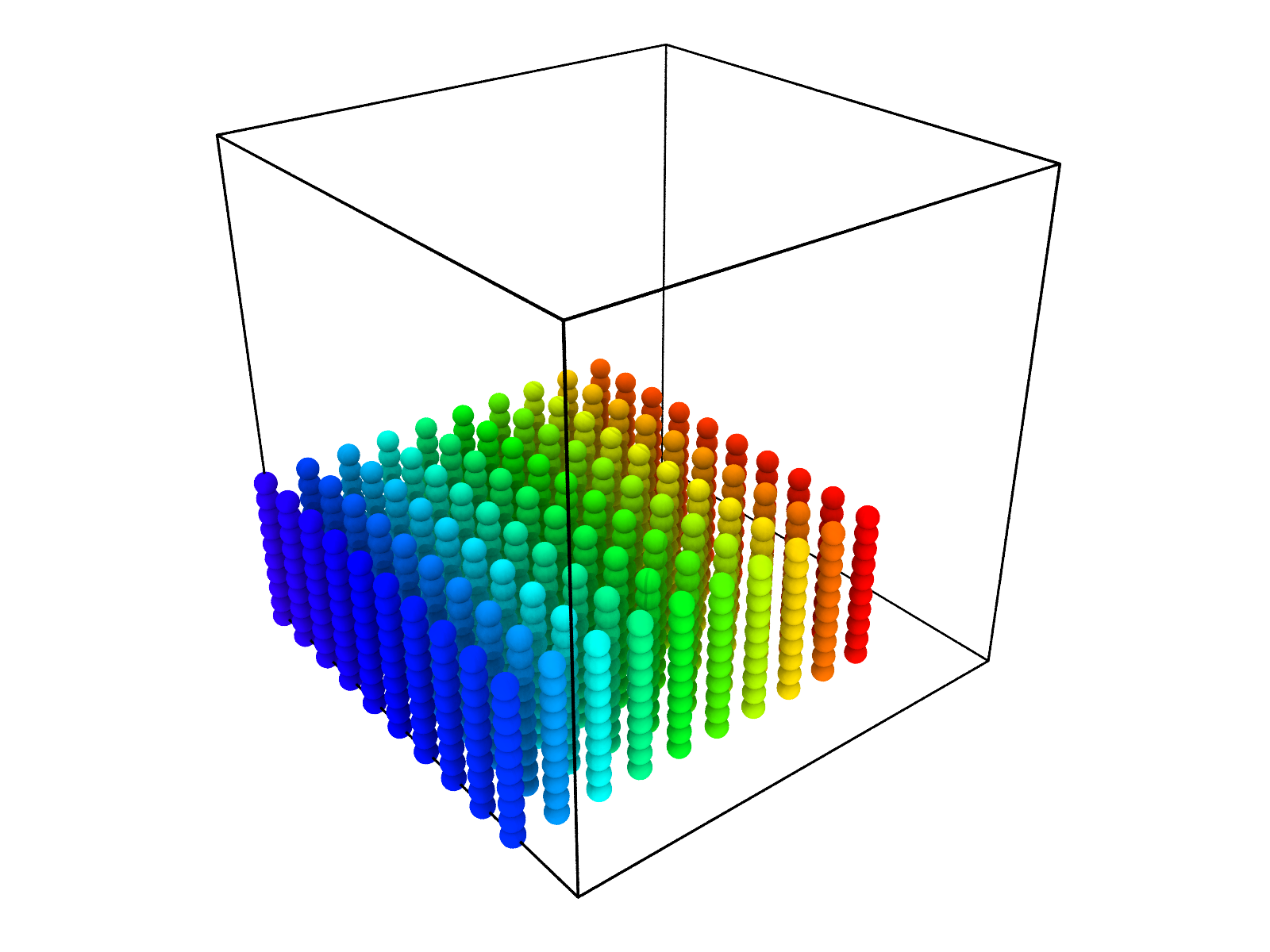

Defining the force field

We will cover two methods for defining the forcefield:

1. Using the Python API.

2. Creating a forcefield xml file.

Both methods achieve the same result of defining the forcefield. There are pros and cons of both ways. The key points are that using the Python API is more flexible, while creating a forcefield xml file makes it easier to share your forcefield and helps reproducibility. This is demonstrated in the other OpenMM tutorials — the standard forcefields such as Amber are distributed with OpenMM as xml files, while the custom forces used to do free energy calculations are defined using the Python API.

Defining a force-field using the Python API

We can create instances of the OpenMM Force classes, assign parameters, and add them to the system. First we must create a System.

# create the system and add the particles to it
system = mm.System()
system.setDefaultPeriodicBoxVectors(*topology.getPeriodicBoxVectors())
for atom in topology.atoms():
    system.addParticle(atom.element.mass)

We will then create a HarmonicBondForce and a CustomNonBondedForce.

For each bond that is defined in the topology we need to add it to the HarmonicBondForce. We set the equilibrium bond lengths and spring constants to be 0.38 nm and 1000 kJ/mol/nm respectively which are consistent with parameters used in amino-acid level CG models [1].

We define the CustomNonBondedForce to be a Lennard-Jones interaction. We set the value of sigma to be 0.5nm to approximate the size of an amino acid and the value of epsilon to 1 kJ/mol to create a potential that is attractive at 300K. Please do not use these parameters for real simulations. You should consult the literature and choose an appropriate CG force-field or systematically create your own parameter set! Finally, we add exclusions between atoms that are directly bonded and set a cutoff of 1.5nm.

Note that because we have defined a Lennard-Jones potential we could have used the standard `NonBondedForce <http://docs.openmm.org/latest/api-python/generated/openmm.openmm.NonbondedForce.html#openmm.openmm.NonbondedForce>`__, but to demonstrate the flexibility to use different user defined potentials we have used CustomNonBondedForce.

harmonic_bond_force = mm.HarmonicBondForce()

# Add each bond to the force from the topology
for bond in topology.bonds():
    harmonic_bond_force.addBond(bond.atom1.index, bond.atom2.index, 0.38, 1000)

# Define a Lennard-Jones potential
expression = '4*epsilon*((sigma/r)^12-(sigma/r)^6);'\
            + ' sigma=0.5*(sigma1+sigma2);'\
            + ' epsilon=sqrt(epsilon1*epsilon2)'

custom_nb_force = mm.CustomNonbondedForce(expression)

custom_nb_force.addPerParticleParameter('sigma')
custom_nb_force.addPerParticleParameter('epsilon')

# Add the parameters for each particle
for atom in topology.atoms():
    custom_nb_force.addParticle([0.5, 1.0])

# Create exclusions for directly bonded atoms
custom_nb_force.createExclusionsFromBonds([(bond[0].index, bond[1].index) for bond in topology.bonds()], 1)

# Set a cutoff of 1.5nm
custom_nb_force.setNonbondedMethod(mm.CustomNonbondedForce.CutoffPeriodic)
custom_nb_force.setCutoffDistance(1.5*unit.nanometers)

# Add the forces to the system
system.addForce(harmonic_bond_force)
system.addForce(custom_nb_force)

The system is now ready to simulate. Before we run the simulation we will describe the other method of defining a forcefield by creating a custom forcefield xml file.

Creating a force-field xml file

Alternatively, we can create a custom force-field xml file for our system. You should look here first for the full information: http://docs.openmm.org/latest/userguide/application/05_creating_ffs.html.

You will need to create a new file called “cg_ff.xml” using a text editor of your choice. Then paste the following lines into it:

<!-- cg_ff.xml
Coarse-grained forcefield for a bead-spring polymer. -->
<ForceField>

    <AtomTypes>
        <Type name="CG-bead" class="CG-bead" element="CG" mass="120.0"/>
    </AtomTypes>

    <Residues>
        <!-- Each bead is a single residue.
        Need a template for the different Residue types.
        First type is the end. This only has one bond. -->
        <Residue name="CG-residue-end">
            <Atom name="CG-bead" type="CG-bead"/>
            <ExternalBond atomName="CG-bead"/>
        </Residue>

        <!-- Second type is in the middle of the chain. This has two bonds. -->
        <Residue name="CG-residue-middle">
            <Atom name="CG-bead" type="CG-bead"/>
            <ExternalBond atomName="CG-bead"/>
            <ExternalBond atomName="CG-bead"/>
        </Residue>
    </Residues>

    <!-- Define a harmonic bond between the CA-beads -->
    <HarmonicBondForce>
        <Bond class1="CG-bead" class2="CG-bead" length="0.38" k="1000.0"/>
    </HarmonicBondForce>

    <!-- Use a custom non-bonded force for maximum flexibility.
    The bondCutoff=1 tells it to only exclude interactions between directly bonded atoms. -->
    <CustomNonbondedForce energy="4*epsilon*((sigma/r)^12-(sigma/r)^6); sigma=0.5*(sigma1+sigma2); epsilon=sqrt(epsilon1*epsilon2)" bondCutoff="1">
        <PerParticleParameter name="sigma"/>
        <PerParticleParameter name="epsilon"/>
        <Atom type="CG-bead" sigma="0.5" epsilon="1.0"/>
    </CustomNonbondedForce>
</ForceField>

(If you have cloned the cookbook repo then this file will already exist) The comments in the above code explain what the difference sections are for.

Create the system

We can now load in our previously created custom ForceField and use the createSystem method with the topology.

# load in the ForceField we created
ff = app.ForceField('./cg_ff.xml')
system2 = ff.createSystem(topology, nonbondedMethod=app.CutoffPeriodic, nonbondedCutoff=1.5*unit.nanometers)

We can compare the two systems to check if they are the same. A simple way to do this is to serialize the systems as save them as xml files.

with open('system1.xml', 'w') as output:
    output.write(mm.XmlSerializer.serialize(system))

with open('system2.xml', 'w') as output:
    output.write(mm.XmlSerializer.serialize(system2))

!diff system1.xml system2.xml

We actually find they are slightly different. system2 created by ForceField.createSystem has a CMMotionRemover that was added by default when using the createSystem method. If we wanted to we could add this to the first system.

Setup and run the simulation

We will use a LangevinMiddleIntegrator with a friction term of 0.01ps^-1 and a timestep of 0.01ps as used in similar coarse-grained polymer models [1]. For your own models these parameters will be important and you will need to choose them carefully!

integrator = mm.LangevinMiddleIntegrator(300*unit.kelvin, 0.01/unit.picosecond, 0.010*unit.picoseconds)
simulation = app.Simulation(topology, system, integrator)
simulation.context.setPositions(positions)

# setup simulation reporters
# Write the trajectory to a file called 'traj.dcd'
simulation.reporters.append(app.DCDReporter('traj.dcd', 1000, enforcePeriodicBox=False))

# Report information to the screen as the simulation runs
simulation.reporters.append(app.StateDataReporter(stdout, 1000, step=True,
        potentialEnergy=True, temperature=True, volume=True, speed=True))


# NVT equilibration
simulation.step(10000)

# Add a barostat
barostatIndex=system.addForce(mm.MonteCarloBarostat(1.0*unit.bar, 300*unit.kelvin))
simulation.context.reinitialize(preserveState=True)

# Run NPT equilibration
simulation.step(100000)


# output the equilibrated configuration
with open('equilibrated_config.pdb','w') as f:
    state = simulation.context.getState(getPositions=True, enforcePeriodicBox=True)
    topology.setPeriodicBoxVectors(state.getPeriodicBoxVectors())
    app.PDBFile.writeFile(topology, state.getPositions(), f)

The equilibrated system will be a polymer melt that looks similar to this: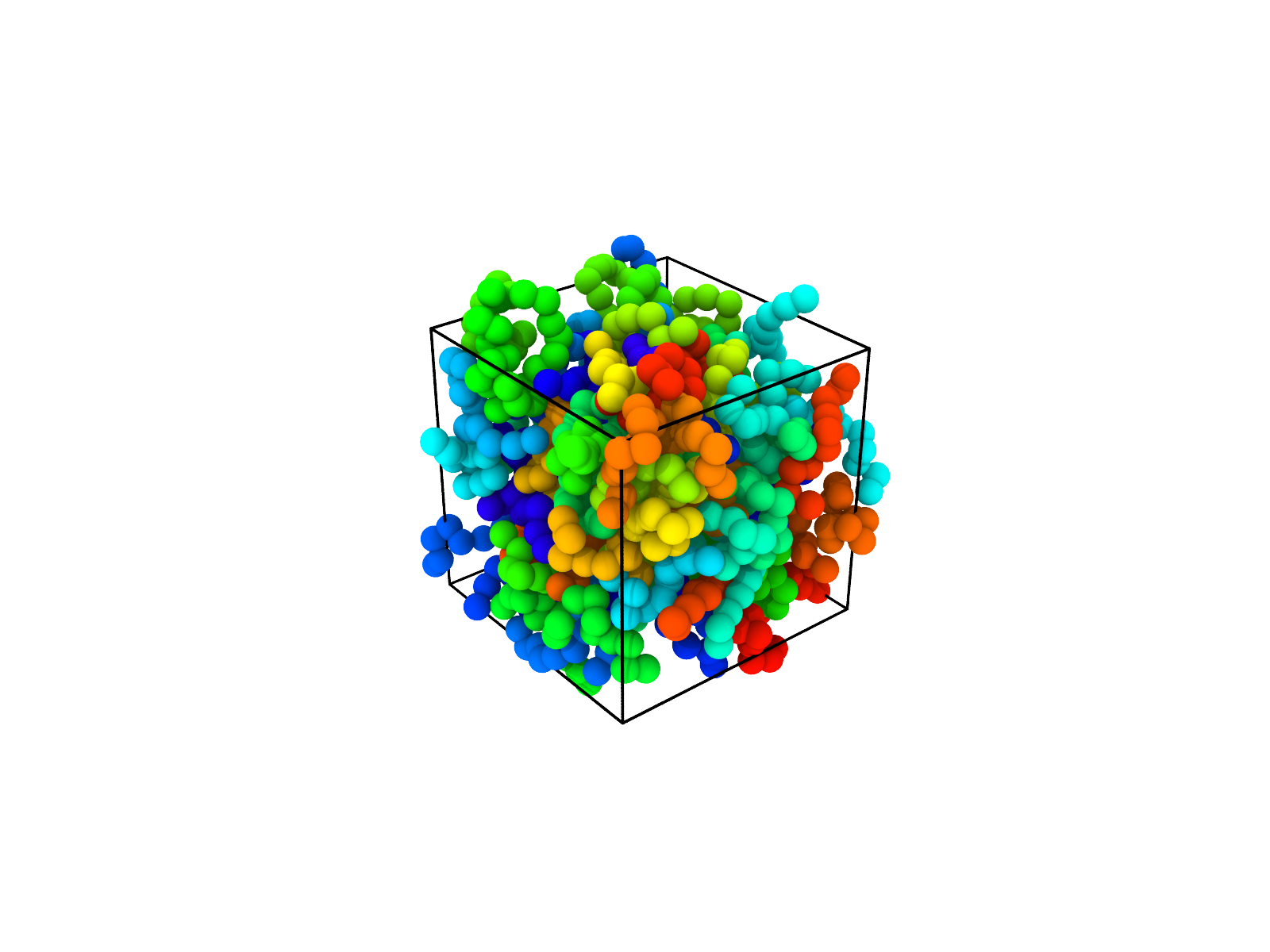

References

[1] GL Dignon, W Zheng, YC Kim, RB Best, J Mittal, PLoS computational biology 14 (1), 2018. https://doi.org/10.1371/journal.pcbi.1005941