Protein in Water
Solvating a protein structure from the PDB and running NPT dynamics
Introduction
This is the OpenMM version of Justin A. Lemkul’s Lysozyme in Water GROMACS tutorial.
It will cover the following steps
Load a PDB file into OpenMM
Choose the force-field
Clean-up the file
Solvate the protein with water and ions
Setup system and integrator
Run local minization
Run NVT equilibration
Run NPT production molecular dynamics
Basic analysis.
Download the protein structure file
First we need to download the PDB file of the lysozome from the RCSB Protein Data Bank https://www.rcsb.org/structure/1aki
[1]:
!wget https://files.rcsb.org/download/1AKI.pdb
--2022-12-23 14:47:36--  https://files.rcsb.org/download/1AKI.pdb
Resolving files.rcsb.org (files.rcsb.org)... 128.6.158.66
Connecting to files.rcsb.org (files.rcsb.org)|128.6.158.66|:443... connected.
HTTP request sent, awaiting response... 200 OK
Length: unspecified [application/octet-stream]
Saving to: ‘1AKI.pdb’

1AKI.pdb                [  <=>               ] 113.59K   456KB/s    in 0.2s

2022-12-23 14:47:40 (456 KB/s) - ‘1AKI.pdb’ saved [116316]
Load the PDB file into OpenMM
[2]:
from openmm.app import *
from openmm import *
from openmm.unit import *
from sys import stdout

pdb = PDBFile("1AKI.pdb")
Define the forcefield
We need to define the forcefield we want to use. We will use the Amber14 forcefield and the TIP3P-FB water model.
[3]:
# Specify the forcefield
forcefield = ForceField('amber14-all.xml', 'amber14/tip3pfb.xml')
Clean up
This PDB file contains some crystal water molecules which we want to strip out. This can be done using the Modeller class. We also add in any missing H atoms.
[4]:
modeller = Modeller(pdb.topology, pdb.positions)
modeller.deleteWater()
residues=modeller.addHydrogens(forcefield)
Solvate
We can use the addSolvent method to add water molecules
[5]:
modeller.addSolvent(forcefield, padding=1.0*nanometer)
This command creates a box that has edges at least 1nm away from the solute and fills it with water molecules. Addionally it adds in the required number of CL and Na ions to make the system charge neutral.
Setup system and Integrator
We now need to combine our molecular topology and the forcefield to create a complete description of the system. This is done using the ForceField object’s createSystem() function. We then create the integrator, and combine the integrator and system to create the Simulation object. Finally we set the initial atomic positions.
[6]:
system = forcefield.createSystem(modeller.topology, nonbondedMethod=PME, nonbondedCutoff=1.0*nanometer, constraints=HBonds)
integrator = LangevinMiddleIntegrator(300*kelvin, 1/picosecond, 0.004*picoseconds)
simulation = Simulation(modeller.topology, system, integrator)
simulation.context.setPositions(modeller.positions)
Local energy minimization
It is a good idea to run local energy minimization at the start of a simulation, since the coordinates in the PDB file might produce very large forces
[7]:
print("Minimizing energy")
simulation.minimizeEnergy()
Minimizing energy
Setup reporting
To get output from our simulation we can add reporters. We use PDBReporter to write the coorinates every 1000 timesteps to “output.pdb” and we use StateDataReporter to print the timestep, potential energy, temperature, and volume to the screen and to a file called “md_log.txt”.
[8]:
simulation.reporters.append(PDBReporter('output.pdb', 1000))
simulation.reporters.append(StateDataReporter(stdout, 1000, step=True,
        potentialEnergy=True, temperature=True, volume=True))
simulation.reporters.append(StateDataReporter("md_log.txt", 100, step=True,
        potentialEnergy=True, temperature=True, volume=True))
NVT equillibration
We are using a Langevin integrator which means we are simulating in the NVT ensemble. To equilibrate the temperature we just need to run the simulation for a number of timesteps.
[9]:
print("Running NVT")
simulation.step(10000)
Running NVT
#"Step","Potential Energy (kJ/mole)","Temperature (K)","Box Volume (nm^3)"
1000,-361152.47182837734,290.59113263667587,237.5626678984939
2000,-358285.09682837734,302.79078945563003,237.5626678984939
3000,-358005.84682837734,302.48286620646525,237.5626678984939
4000,-358507.72182837734,298.6930169859535,237.5626678984939
5000,-358184.97182837734,299.2717701713331,237.5626678984939
6000,-358212.97182837734,300.75294253983,237.5626678984939
7000,-359764.59682837734,300.86799019463365,237.5626678984939
8000,-358504.22182837734,300.08571555582586,237.5626678984939
9000,-358743.72182837734,301.49754076972073,237.5626678984939
10000,-358427.47182837734,303.0196359235443,237.5626678984939
NPT production MD
To run our simulation in the NPT ensemble we need to add in a barostat to control the pressure. We can use MonteCarloBarostat.
[10]:
system.addForce(MonteCarloBarostat(1*bar, 300*kelvin))
simulation.context.reinitialize(preserveState=True)


print("Running NPT")
simulation.step(10000)
Running NPT
11000,-360868.2039845481,296.6271613599709,229.55243059554863
12000,-360440.69597966364,299.2972740816768,227.9584335998326
13000,-360306.2146281218,298.81725153096374,226.29494575252173
14000,-361092.9398954578,303.07884143773134,225.42478987487024
15000,-360441.3635788809,300.7599116506667,225.36581137758682
16000,-360902.0646238751,298.85839880440795,224.7134712811861
17000,-361590.4094829492,298.67191986774935,224.97738234573134
18000,-360249.67117970064,296.2367386071592,224.69872883856726
19000,-360755.6596395951,302.12766052941635,224.73491745579543
20000,-361129.44742261735,298.26462186445406,225.16297011700198
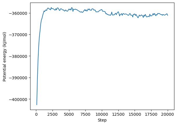
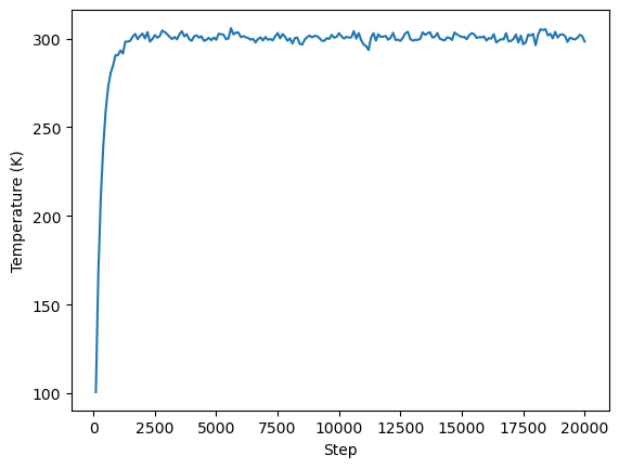
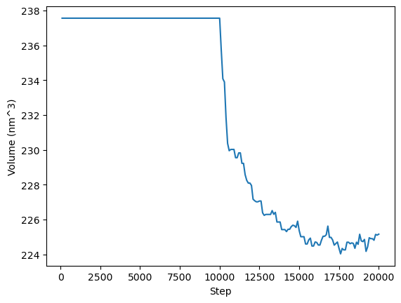
Analysis
We can now do some basic analysis using Python. We will plot the time evolution of the potential energy, temperature, and box volume. Remember that OpenMM itself is primarly an MD engine, for in-depth anaylsis of your simulations you can use other python packages such as MDtraj, or MDAnalysis.
[11]:
import numpy as np
import matplotlib.pyplot as plt
data = np.loadtxt("md_log.txt", delimiter=',')

step = data[:,0]
potential_energy = data[:,1]
temperature = data[:,2]
volume = data[:,3]

plt.plot(step, potential_energy)
plt.xlabel("Step")
plt.ylabel("Potential energy (kJ/mol)")
plt.show()
plt.plot(step, temperature)
plt.xlabel("Step")
plt.ylabel("Temperature (K)")
plt.show()
plt.plot(step, volume)
plt.xlabel("Step")
plt.ylabel("Volume (nm^3)")
plt.show()